LLM 推理基础：矩阵乘法并行化

2026-04-17 4 min

目录相关

本文简单介绍 GEMM 运算的几种常见的并行计算方式。

在分布式计算场景下，什么时候通信是必须的

对于两个矩阵 $A \in \mathbb{R}^{M \times N}$ 和 $B \times \mathbb{R}^{N \times K}$ ，矩阵计算可以表示为

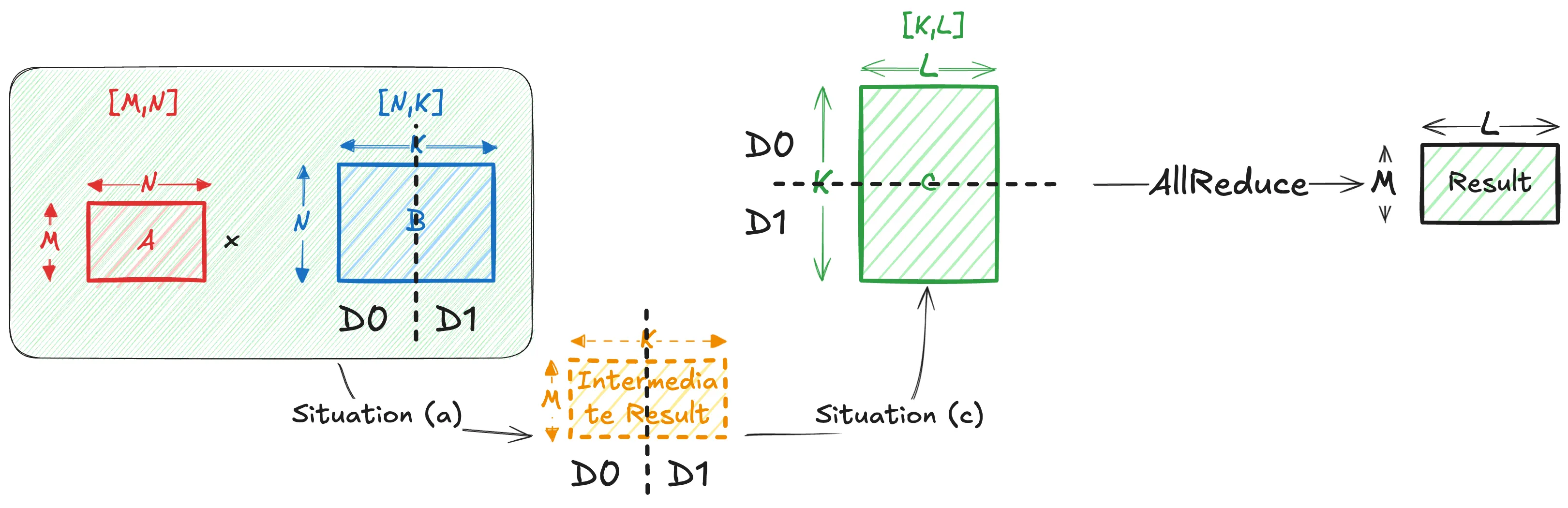
\forall (i, k) \in [\![1, M]\!] \times [\![1, K]\!], \quad C_{ik} = \sum_{j=1}^N A_{ij}B_{jk}

我们可以看到有两种拆分方式：（1） $M$ 和 $K$ 维度的拆分，对应拆分 $C_{i.}$ 和 $C_{.k}$ 的计算，每个 rank 负责一部分 $C_{ik}$ 。计算是相互独立的，除非要重建完整的矩阵，通信是没有必要的（2） $N$ 维度的拆分，这意味着每个 rank 分别负责所有元素的一部分的求和计算。此时一定需要聚合通信，不然的话矩阵的计算结果就不正确。

第二种情况推导：假设设备为 $p$ ，分到一部分的 $J_{p} \subset \{1, \dots, N\}$

C_{ik}^{(p)} = \sum_{j \in J_{p} }A_{ij }B_{jk},\quad C_{ik} = \sum_{p}C_{ik}^{(p)}

结论是在矩阵乘法时，当拆分求和维时就必须需要通信。

两个矩阵乘法

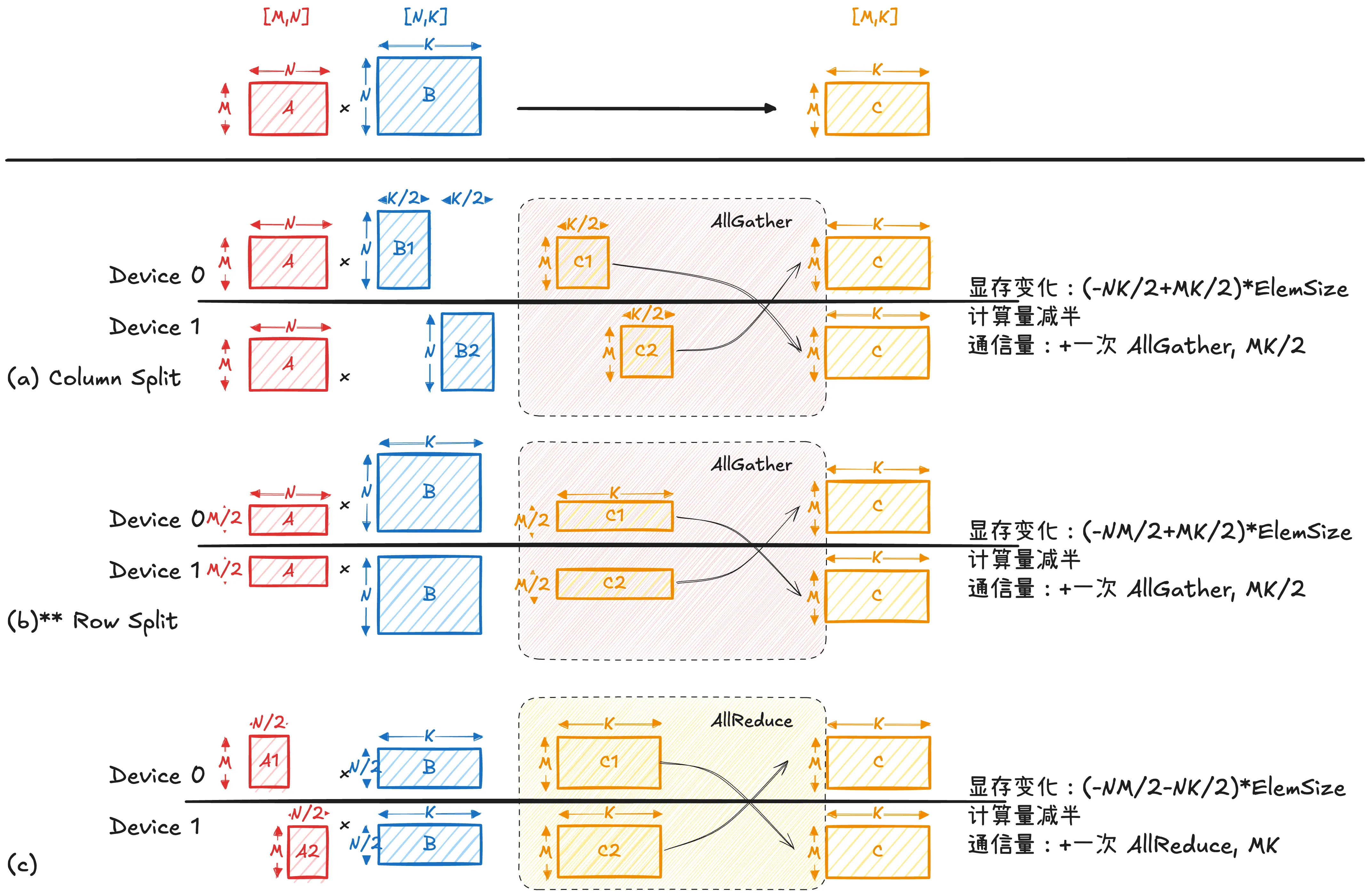
考虑我们需要做以下矩阵乘法的场景：

(A,B) \mapsto AB, \quad A \in \mathbb{R}^{M \times N}, \; B \in \mathbb{R}^{N \times K}

下图 (a)–(c) 展示了三种典型的矩阵切分方式。其核心区别在于：是否对乘法中的求和维度（即 $N$ 维）进行切分。

(a) 列切 B：每个设备负责输出矩阵 C 的一部分列，计算彼此独立，无需通信，但为了得到完整的输出矩阵需要进行一次 AllGather。
(b) 行切 A：每个设备负责输出矩阵 C 的一部分行，同样无需通信，但为了得到完整的输出矩阵需要进行一次 AllGather。该方式在神经网络推理中最为常见（例如 activation 按 batch 或 token 维切分）。
(c) 列切 A 且行切 B：等价于对乘法中的求和维度进行切分，每个设备仅计算部分乘加结果（partial sum），最终必须需要通过 AllReduce 完成结果合并。这种方式具有更高的并行粒度，但会引入额外通信开销。

参考代码实现

# Code for (a)
import numpy as np
M, N, K = 4, 16, 8

A = np.random.randint(0, 10, size=(M, N))
B = np.random.randint(0, 10, size=(N, K))
print("Matrix A shape:", A.shape)
print("Matrix B shape:", B.shape)

num_splits = 4
assert K % num_splits == 0, "K must be divisible by num_splits"
B_splits = np.split(B, num_splits, axis=1)
for i, B_split in enumerate(B_splits):
    print(f"Split {i} shape: {B_split.shape}")

# Distributed computation of A @ B using splits of B
local_results = [A @ B_split for B_split in B_splits]
for i, local_result in enumerate(local_results):
    print(f"Local result {i} shape: {local_result.shape}")

# Assemble the final result: AllGather
C_final = np.hstack(local_results)
# equivalent to C_final = np.concatenate(local_results, axis=1)
print("Final result shape:", C_final.shape)

三个矩阵乘法

现在考虑到我们需要做三个矩阵乘法，即：

(A,B,C) \mapsto ABC, \quad A \in \mathbb{R}^{M \times N}, \; B \in \mathbb{R}^{N \times K}, \; C \in \mathbb{R}^{K \times L}

常见的方法是 列切 B + 行切 C。

第一步 $AB$ 计算类似上一小节 (a)，得到列切的输出
再运用上一小节 (c)，与行切 $C$ 计算，再经过 AllReduce 得到完整输出